

最小二乗法を使用して、楕円フィッティングを行うアルゴリズムについて考えてみます。
うまくいけば、量子化誤差の壁を越えて細胞の形態学的解析に応用できそうです。
目次
偏微分を使用した最小二乗法
直線の最小二乗法を偏微分を使用して行ってみます。
初めに、
$$e:\sum_{i}( y_i-(ax_i)+b))^2$$
について、eを最小化するa,bについて考えます。
上記の式を展開すると、
$$e:\sum_{i}e_i^2$$
$e_i = a^2x_i^2+2ax_ib+b^2-2ax_iy_i-2by_i+y_i^2$
この時、
$$\frac{\partial e}{\partial a} =2a\sum_{i} x_i^2+2b\sum_{i}x_i-2\sum_{i}x_iy_i$$
$$\frac{\partial e}{\partial b}= 2a\sum_{i}x_i+2b\sum_{i}-2\sum_{i}y_i$$
$$\frac{\partial e}{\partial a}=\frac{\partial e}{\partial b}=0$$
未知数2に対して、2つの方程式があるため、a,bについて解きます。
$\mathbf{W}= \begin{pmatrix} \sum_{i} x_i^2 & \sum_{i} x_i \\ \sum_{i} x_i & n\\ \end{pmatrix}$
$\mathbf{f}=\begin{pmatrix} \sum_{i}x_iy_i \\ \sum_{i}y_i \\ \end{pmatrix}$
$\mathbf{c} = \begin{pmatrix} a \\ b\\ \end{pmatrix}$
$\mathbf{W} \mathbf{c} =\mathbf{f}$
$\mathbf{c} =(\mathbf{W} ^{\mathrm{T}}\mathbf{W})^{-1}\mathbf{W} ^{\mathrm{T}}\mathbf{f}$
(今回は$\mathbf{W}$が正則なので、わざわざ転置行列を計算する必要はないですが、一般化しておきます。)
Pythonで実装
import matplotlib.pyplot as plt
import numpy as np
from numpy.linalg import solve

fig = plt.figure()

X = [3*i for i in range(1,11)]
Y = [5,8,11,20,25,31,33,43,45,51]

A = np.array([[i,1] for i in X])
c = np.transpose(np.array(Y))
A_t = np.transpose(A)

left = A_t@A
right = A_t@c
d  = solve(left,right)
print(d)

y_hat = [i*d[0]+d[1] for i in X]
plt.scatter(X,Y,color = "black")
plt.plot(X,y_hat,color = 'black')


sum_x2, sum_x, sum_xy, sum_y, n = 0, 0, 0, 0, 0

for i in range(len(X)):
    sum_x += X[i]
    sum_x2 += X[i]**2
    sum_xy += X[i]*Y[i]
    sum_y += Y[i]
    n += 1

W = np.array([[sum_x2,sum_x],[sum_x,n]])
W_t = np.array(W)
f = np.transpose(np.array([sum_xy,sum_y]))

d = np.linalg.inv(W_t@W)@W_t@f
print(d)

y_hat = [i*d[0]+d[1] for i in X]
plt.plot(X,y_hat,color = 'orange')

plt.xlabel("X")
plt.ylabel("f")
plt.grid()
fig.savefig("blog.png",dpi = 500)
>>>
[ 1.77373737 -2.06666667]
[ 1.77373737 -2.06666667]
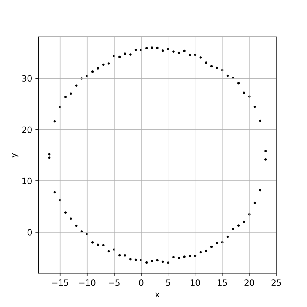
円の方程式に対するL2ノルム最小化
いきなり楕円に行くと複雑なので、一旦シンプルな円で考えてみます。
以下の円の方程式を使用して、Pythonで描画します。
$$(x-a)^2+(y-b)^2 = r^2$$
import numpy as np
import matplotlib.pyplot as plt
import random
fig = plt.figure(figsize=[5,5])

a = 3
b = 4
plt.plot(a,b)
r = 20

x = [i for i in range(-(r-a),(r+b))]
print(len(x))

y_p = [np.sqrt(r**2-(i-a)**2)+b +random.random()+11 for i in x]
y_n = [-np.sqrt(r**2-(i-a)**2)+b +random.random()+10 for i in x]

print(y_p)
plt.scatter(x,y_p,s = 3,color = 'black')
plt.scatter(x,y_n,s = 3,color = 'black')

# plt.plot(x,y_p,color= "black")
# plt.plot(x,y_n,color= "black")

plt.grid()
plt.xlabel("x")
plt.ylabel("y")

fig.savefig("a.png",dpi = 500)
上記の円の方程式について、
$$e:\sum_{i}e_i^2$$
$e_i = (x_i-a)^2+(y_i-b)^2 – r^2$
を最小化するa,b,rについて考えます。
この時、
$C_1 = -2a,\:\:C_2=-2b, \:\: C_3 = a^2+b^2-r^2,\:\:C_i\in \mathbb{R}$
とおくと、
$e_i = (x_i^2+y_i^2+C_1x_i+C_2y_i+C_3)^2$
偏微分で最小化
$$\frac{\partial e}{\partial C_1} =C_1\sum_{i} x_i^2+C_2\sum_{i} x_iy_i+C_3\sum_{i} x_i^3+\sum_{i} x_iy_i^2$$
$$\frac{\partial e}{\partial C_2} = C_1\sum_{i}x_iy_i+C_2\sum_{i} y_i^2+C_3y_i+\sum_{i} x_i^2y_i+\sum_{i} y_i^3 $$
$$\frac{\partial e}{\partial C_3} = C_1\sum_{i}x_i+C_2\sum_{i}y_i+C_3n+\sum_{i}x_i^2+\sum_{i}y_i^2 $$
$$\frac{\partial e}{\partial C_1}=\frac{\partial e}{\partial C_2}=\frac{\partial e}{\partial C_3}=0$$
行列表示すると、
$\mathbf{W}=\begin{pmatrix}\sum_{i}x_i^2 & \sum_{i}x_iy_i &\sum_{i}x_i\\\sum_{i}x_iy_i & \sum_{i}y_i^2&\sum_{i}y_i\\\sum_{i}x_i & \sum_{i}y_i&n\end{pmatrix}$
$\mathbf{c} = \begin{pmatrix} C_1 \\ C_2\\C_3 \end{pmatrix}$
$\mathbf{f} = \begin{pmatrix} -\sum_{i}x_i^3-\sum_{i}x_i y_i^2\\ -\sum_{i}x_i^2y_i-\sum_{i}y_i^3\\-\sum_{i} x_i^2 – \sum_{i} y_i^2 \end{pmatrix}$
$\mathbf{W} \mathbf{c} =\mathbf{f}$
$\mathbf{c} =(\mathbf{W} ^{\mathrm{T}}\mathbf{W})^{-1}\mathbf{W} ^{\mathrm{T}}\mathbf{f}$
正規方程式で最小化
$x_i^2+y_i^2+C_1x_i+C_2y_i+C_3$
について、以下のような正規方程式を作成します。
$ \begin{pmatrix} x_1&y_1 & 1\\ \vdots&\vdots &\vdots\\ x_i&y_i & 1 \end{pmatrix} \begin{pmatrix} C_1 \\ C_2\\C_3 \end{pmatrix}= \begin{pmatrix} -x_1^2-y_1^2 \\ \vdots\\-x_i^2-y_i^2 \end{pmatrix}$
よって、
$\mathbf{A}\mathbf{c}=\mathbf{b}$
$\mathbf{c} = (\mathbf{A} ^{\mathrm{T}}\mathbf{A})^{-1}\mathbf{A} ^{\mathrm{T}}\mathbf{b}$
Pythonで実装
正規方程式の方がシンプルなので、そちらで実装してみます。
import numpy as np
import matplotlib.pyplot as plt
import random
from numpy.linalg import solve
fig = plt.figure(figsize=[7,5])
a = 3
b = 4
r = 20
x = [i for i in range(-(r-a),(r+b))]
print(len(x))
y_p = [np.sqrt(r**2-(i-(a))**2)+b +random.random() for i in x]
plt.scatter(x,y_p,s = 15,color = 'black')
x = [i for i in range(-(r-a),(r+b))]
y = y_p
A = np.transpose(np.array([[i for i in x],[i for i in y],[1 for i in range(len(x))]]))
A_t = np.transpose(A)
f = np.array([-i**2 -j**2 for i,j in zip(x,y)])
f = np.transpose(f)
print(A)
left = A_t@A
right = A_t@f
d = solve(left,right)
print(d)
C_1, C_2, C_3 = d[0], d[1], d[2]
a = C_1/(-2)
b = C_2/(-2)
r = np.sqrt(a**2+b**2-C_3)
print(a,b,r)
y_p = [np.sqrt(r**2-(i-a)**2)+b for i in x]
y_n = [-i+2*b for i in y_p]
plt.scatter(x,y_p,color = 'orange',s= 15)
plt.grid()
plt.xlabel("x")
plt.ylabel("y")
fig.savefig("a.png",dpi = 500)
>>>
[[-17. 4.69456925 1. ]
[-16. 11.23082097 1. ]
[-15. 13.33797773 1. ]
[-14. 15.45430748 1. ]
[-13. 16.99308676 1. ]
[-12. 17.57940836 1. ]
[-11. 18.58066499 1. ]
[-10. 19.2939066 1. ]
[ -9. 20.94187394 1. ]
[ -8. 21.20180011 1. ]
[ -7. 21.79644929 1. ]
[ -6. 22.64014597 1. ]
[ -5. 23.03803291 1. ]
[ -4. 22.95555662 1. ]
[ -3. 23.72394048 1. ]
[ -2. 24.14147832 1. ]
[ -1. 23.98613516 1. ]
[ 0. 24.58386085 1. ]
[ 1. 24.76505385 1. ]
[ 2. 24.71697776 1. ]
[ 3. 24.56786747 1. ]
[ 4. 24.81799425 1. ]
[ 5. 24.03217142 1. ]
[ 6. 23.87453316 1. ]
[ 7. 24.57538764 1. ]
[ 8. 23.78170807 1. ]
[ 9. 23.594457 1. ]
[ 10. 23.51572552 1. ]
[ 11. 23.04827775 1. ]
[ 12. 22.11196693 1. ]
[ 13. 21.52661483 1. ]
[ 14. 21.53137029 1. ]
[ 15. 20.84882428 1. ]
[ 16. 19.76258791 1. ]
[ 17. 18.91608725 1. ]
[ 18. 17.35368547 1. ]
[ 19. 16.53268051 1. ]
[ 20. 14.59907094 1. ]
[ 21. 13.67109722 1. ]
[ 22. 10.69635721 1. ]
[ 23. 4.63834337 1. ]]
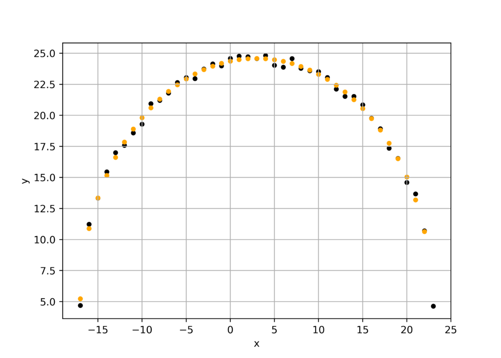
[ -5.92207979 -9.23264149 -368.74515149]
2.9610398934439273 4.616320746541363 19.970561483657104オレンジの点がL2ノルムを最小化したものです。
楕円フィッテング
楕円の一般式は以下のように与えられます。
$\frac{(x-p)^2}{a^2} + \frac{(y-q)^2}{b^2} =1$
ここで、
$C_1 = -2p$
$C_2 = -2q\frac{a^2}{b^2}$
$C_3 = \frac{a^2}{b^2}$
$C_4 = p^2+\frac{a^2}{b^2}q^2-a^2$
とすると、
$ \begin{pmatrix} x_1&y_1 &y_1^2& 1\\ \vdots&\vdots &\vdots&\vdots\\ x_i&y_i &y_i^2& 1 \end{pmatrix} \begin{pmatrix} C_1 \\ C_2\\C_3\\C_4 \end{pmatrix}= \begin{pmatrix} -x_1^2 \\ \vdots\\-x_i^2\end{pmatrix}$
よって正規方程式を以下のように解くと、未知の4変数を得ることができます。
$\mathbf{c} = (\mathbf{A} ^{\mathrm{T}}\mathbf{A})^{-1}\mathbf{A} ^{\mathrm{T}}\mathbf{b}$
Pythonで実装
import numpy as np
import matplotlib.pyplot as plt
import random
from numpy.linalg import solve
fig = plt.figure(figsize=[10,5])

p = 10
q = 15
a = 10
b = 5

x = [i for i in range((p-a),(p+a)+1)]
y = [np.sqrt(b**2-b**2/a**2*(i-p)**2)+q +random.random() for i in x]
print(y)
plt.scatter(x,y,s=15,color = "black")

A = np.transpose(np.array([[float(i) for i in x],[float(i) for i in y],[float(i**2)for i in y],[float(1) for i in x]]))
A_t = np.transpose(A)
B = [-float(i**2) for i in x]

left = A_t@A
right = A_t@B
d  = solve(left,right)
print(d)
print(p,q,a,b)
C_1, C_2, C_3, C_4 = d[0], d[1], d[2], d[3]
p = -C_1/(2)
q = -C_2/2/C_3
a = np.sqrt(abs(p**2+C_3*q**2-C_4))
b = np.sqrt(a**2/C_3)
print(p,q,a,b)
plt.scatter(x,[np.sqrt(b**2-b**2/a**2*(i-p)**2)+q for i in x],s = 10,color = "orange")
plt.grid()
plt.xlabel("x")
plt.ylabel("y")
fig.savefig("a.png",dpi = 500)
>>>
[15.845269795573678, 17.712951732039468, 18.143931608197057, 19.49209847417363, 19.267284154510413, 20.07616269361377, 19.954894885666462, 20.013130909887085, 20.647374023580767, 20.70059888453033, 20.11776290331141, 20.213796397635615, 20.234422151435872, 20.386809409144664, 20.38337579203502, 19.880791189904308, 19.78039455899217, 19.381828356753733, 18.085496970318214, 17.274689654329972, 15.37057345760351]
[-19.97964006 -87.4999272    2.96813395 642.58052398]
10 15 10 5
9.989820030137787 14.739888559194851 10.103740305630863 5.864627427426599
