
細胞の軸を解析的に決定することができると、大きさや各種局在の定量化に便利です。今回は、以下の記事で、分散共分散行列の固有空間の基底を取得できているので、これを利用して細胞の軸を解析的に決定する方法について考えてみます。
目次
細胞情報の用意
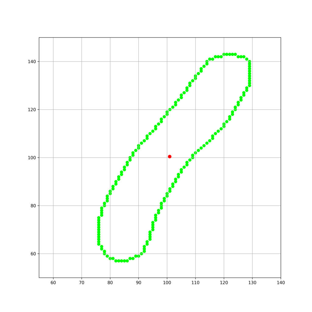
以下のような輪郭座標で構成される細胞について考えます。
cell = [[82, 57], [81, 58], [80, 58], [79, 59], [78, 60], [78, 61], [77, 62], [77, 63], [76, 64], [76, 65], [76, 66], [76, 67], [76, 68], [76, 69], [76, 70], [76, 71], [76, 72], [76, 73], [76, 74], [76, 75], [77, 76], [77, 77], [77, 78], [77, 79], [78, 80], [78, 81], [79, 82], [79, 83], [79, 84], [80, 85], [80, 86], [81, 87], [81, 88], [82, 89], [82, 90], [83, 91], [83, 92], [84, 93], [84, 94], [85, 95], [85, 96], [86, 97], [86, 98], [87, 99], [87, 100], [88, 101], [88, 102], [89, 103], [90, 104], [90, 105], [91, 106], [92, 107], [93, 108], [93, 109], [94, 110], [95, 111], [96, 112], [96, 113], [97, 114], [98, 115], [98, 116], [99, 117], [100, 118], [100, 119], [101, 120], [102, 121], [103, 122], [103, 123], [104, 124], [105, 125], [105, 126], [106, 127], [107, 128], [107, 129], [108, 130], [108, 131], [109, 132], [110, 133], [110, 134], [111, 135], [112, 136], [112, 137], [113, 138], [114, 139], [114, 140], [115, 141], [116, 141], [117, 142], [118, 142], [119, 142], [120, 143], [121, 143], [122, 143], [123, 143], [124, 143], [125, 142], [126, 142], [127, 142], [128, 141], [129, 140], [129, 139], [129, 138], [129, 137], [129, 136], [129, 135], [129, 134], [129, 133], [129, 132], [129, 131], [129, 130], [128, 129], [128, 128], [127, 127], [127, 126], [126, 125], [126, 124], [125, 123], [125, 122], [124, 121], [124, 120], [123, 119], [123, 118], [122, 117], [122, 116], [121, 115], [120, 114], [120, 113], [119, 112], [118, 111], [117, 110], [116, 109], [116, 108], [115, 107], [114, 106], [113, 105], [112, 104], [111, 103], [110, 102], [109, 101], [109, 100], [108, 99], [107, 98], [107, 97], [106, 96], [105, 95], [105, 94], [104, 93], [104, 92], [103, 91], [103, 90], [102, 89], [102, 88], [101, 87], [101, 86], [100, 85], [100, 84], [99, 83], [99, 82], [98, 81], [98, 80], [98, 79], [97, 78], [97, 77], [96, 76], [96, 75], [96, 74], [95, 73], [95, 72], [95, 71], [95, 70], [94, 69], [94, 68], [94, 67], [94, 66], [93, 65], [93, 64], [92, 63], [92, 62], [92, 61], [91, 60], [90, 59], [89, 59], [88, 58], [87, 58], [86, 57], [85, 57], [84, 57], [83, 57]]これを可視化します。
import matplotlib.pyplot as plt
import numpy as np
from numpy.linalg import eig

cell = [[82, 57], [81, 58], [80, 58], [79, 59], [78, 60], [78, 61], [77, 62], [77, 63], [76, 64], [76, 65], [76, 66], [76, 67], [76, 68], [76, 69], [76, 70], [76, 71], [76, 72], [76, 73], [76, 74], [76, 75], [77, 76], [77, 77], [77, 78], [77, 79], [78, 80], [78, 81], [79, 82], [79, 83], [79, 84], [80, 85], [80, 86], [81, 87], [81, 88], [82, 89], [82, 90], [83, 91], [83, 92], [84, 93], [84, 94], [85, 95], [85, 96], [86, 97], [86, 98], [87, 99], [87, 100], [88, 101], [88, 102], [89, 103], [90, 104], [90, 105], [91, 106], [92, 107], [93, 108], [93, 109], [94, 110], [95, 111], [96, 112], [96, 113], [97, 114], [98, 115], [98, 116], [99, 117], [100, 118], [100, 119], [101, 120], [102, 121], [103, 122], [103, 123], [104, 124], [105, 125], [105, 126], [106, 127], [107, 128], [107, 129], [108, 130], [108, 131], [109, 132], [110, 133], [110, 134], [111, 135], [112, 136], [112, 137], [113, 138], [114, 139], [114, 140], [115, 141], [116, 141], [117, 142], [118, 142], [119, 142], [120, 143], [121, 143], [122, 143], [123, 143], [124, 143], [125, 142], [126, 142], [127, 142], [128, 141], [129, 140], [129, 139], [129, 138], [129, 137], [129, 136], [129, 135], [129, 134], [129, 133], [129, 132], [129, 131], [129, 130], [128, 129], [128, 128], [127, 127], [127, 126], [126, 125], [126, 124], [125, 123], [125, 122], [124, 121], [124, 120], [123, 119], [123, 118], [122, 117], [122, 116], [121, 115], [120, 114], [120, 113], [119, 112], [118, 111], [117, 110], [116, 109], [116, 108], [115, 107], [114, 106], [113, 105], [112, 104], [111, 103], [110, 102], [109, 101], [109, 100], [108, 99], [107, 98], [107, 97], [106, 96], [105, 95], [105, 94], [104, 93], [104, 92], [103, 91], [103, 90], [102, 89], [102, 88], [101, 87], [101, 86], [100, 85], [100, 84], [99, 83], [99, 82], [98, 81], [98, 80], [98, 79], [97, 78], [97, 77], [96, 76], [96, 75], [96, 74], [95, 73], [95, 72], [95, 71], [95, 70], [94, 69], [94, 68], [94, 67], [94, 66], [93, 65], [93, 64], [92, 63], [92, 62], [92, 61], [91, 60], [90, 59], [89, 59], [88, 58], [87, 58], [86, 57], [85, 57], [84, 57], [83, 57]]
x = [i[0] for i in cell]
y = [i[1] for i in cell]
center = [np.mean(y),np.mean(x)]
X = np.array([y,x])

fig_n = plt.figure(figsize=(10,10))
plt.xlim(55,140)
plt.ylim(50,150)
plt.scatter(x,y,s = 40,color = "lime")
plt.scatter(center[1],center[0],s = 50,color = "red",zorder = 100)
plt.grid()
fig_n.savefig("contours_raw.png",dpi=300)
plt.close()
実行結果
基底変換
細胞の座標を以下のようなベクトルで表記します。
$$\mathbf{X} = \begin{pmatrix}x_1 & \cdots&x_n \\y_1 &\cdots & y_n\end{pmatrix}^\mathrm{T}\in\mathbb{R}^{n\times 2} $$
この時、
$$\mathbf{Q}= \begin{pmatrix}v_1&v_2\end{pmatrix}$$
$$\mathbf{\Lambda}= \begin{pmatrix}\lambda_1&0\\0&\lambda_2\end{pmatrix}$$
のもとで、分散共分散行列のスペクトル分解は以下のように表されます。
$$ \begin{pmatrix}V[\mathbf{X_1}] &Cov[\mathbf{X_1},\mathbf{X_2}] \\Cov[\mathbf{X_1},\mathbf{X_2}]s & V[\mathbf{X_2}]\end{pmatrix}= \mathbf{Q}\mathbf{\Lambda}\mathbf{Q}^\mathrm{T}$$
よって、細胞輪郭座標群が存在する座標基底を、以下のようにして固有空間の規定に取り替えることができます。
$$\mathbf{U} = \mathbf{Q}^\mathrm{T}\mathbf{X}$$
これをpythonで以下のように実装します。
fig_base_convert = plt.figure(figsize=(10,10))
plt.xlim(80,190)
plt.ylim(-20,90)
plt.grid()
Q = np.array([eigenvectors[0],eigenvectors[1]]) if eigenvectors[1][0] != 0 else np.array([eigenvectors[1],eigenvectors[0]])
contour_U = [Q.transpose()@np.array([j,i]) for i,j in cell]
print(contour_U)
plt.scatter([i[0] for i in contour_U],[i[1] for i in contour_U],s = 30,color = "lime")

fig_base_convert.savefig("contours_base_convert.png",dpi=300)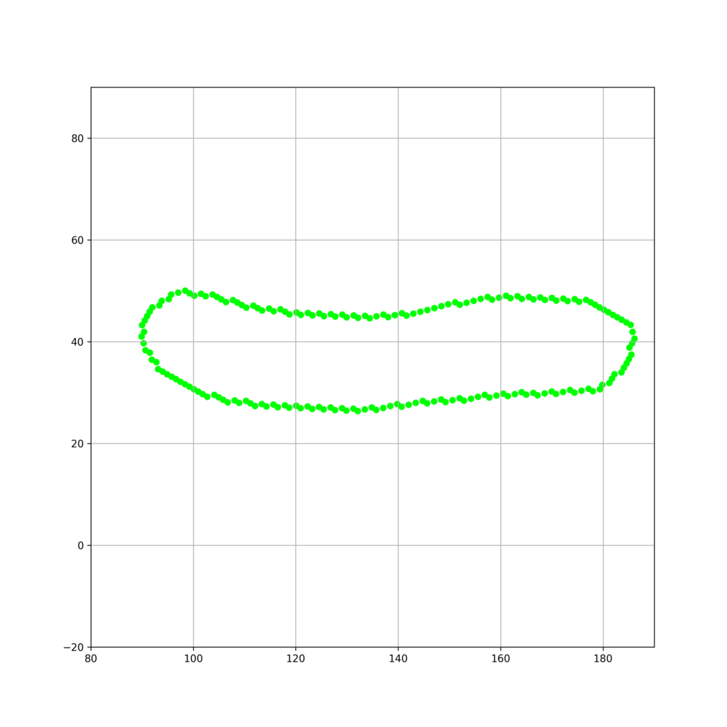
細胞軸の多項式パラメータの決定
基底変換後の各細胞輪郭座標点群を以下のように表します。
$$\mathbf{U} = \begin{pmatrix}u_{1_1} & \cdots&u_{1_n} \\u_{2_1} &\cdots & u_{2_n}\end{pmatrix}^\mathrm{T}\in \mathbb{R}^{n\times 2} $$
この時、任意のk次多項式での回帰は以下のように表すことができます。
$$\mathbf{\theta} = \begin{pmatrix}\theta_0&\cdots&\theta_k\end{pmatrix}^\mathrm{T}\in \mathbb{R}^k$$
$$f\hat{(x)} = \theta^\mathrm{T}\mathbf{X}$$
ここで、正規方程式を組み立てると
$$\mathbf{W}= \begin{pmatrix}u_{11}^k&\cdots&1 \\ \vdots & \vdots & \vdots\\ u_{1n}^k&\cdots&1\end{pmatrix}$$
$$\mathbf{f} = \begin{pmatrix}u_{21}&\cdots&u_{2n}\end{pmatrix}\in \mathbb{R}^n$$
$$\theta = (\mathbf{W}^\mathrm{T}\mathbf{W})^{-1}\mathbf{W}^\mathrm{T}\mathbf{f}$$
上記の式から、細胞軸を表す任意のk次多項式回帰を解析的に行うことができます。
これをpythonで実装します。
import matplotlib.pyplot as plt
import numpy as np
from numpy.linalg import eig, inv
cell = [[82, 57], [81, 58], [80, 58], [79, 59], [78, 60], [78, 61], [77, 62], [77, 63], [76, 64], [76, 65], [76, 66], [76, 67], [76, 68], [76, 69], [76, 70], [76, 71], [76, 72], [76, 73], [76, 74], [76, 75], [77, 76], [77, 77], [77, 78], [77, 79], [78, 80], [78, 81], [79, 82], [79, 83], [79, 84], [80, 85], [80, 86], [81, 87], [81, 88], [82, 89], [82, 90], [83, 91], [83, 92], [84, 93], [84, 94], [85, 95], [85, 96], [86, 97], [86, 98], [87, 99], [87, 100], [88, 101], [88, 102], [89, 103], [90, 104], [90, 105], [91, 106], [92, 107], [93, 108], [93, 109], [94, 110], [95, 111], [96, 112], [96, 113], [97, 114], [98, 115], [98, 116], [99, 117], [100, 118], [100, 119], [101, 120], [102, 121], [103, 122], [103, 123], [104, 124], [105, 125], [105, 126], [106, 127], [107, 128], [107, 129], [108, 130], [108, 131], [109, 132], [110, 133], [110, 134], [111, 135], [112, 136], [112, 137], [113, 138], [114, 139], [114, 140], [115, 141], [116, 141], [117, 142], [118, 142], [119, 142], [120, 143], [121, 143], [122, 143], [123, 143], [124, 143], [125, 142], [126, 142], [127, 142], [128, 141], [129, 140], [129, 139], [129, 138], [129, 137], [129, 136], [129, 135], [129, 134], [129, 133], [129, 132], [129, 131], [129, 130], [128, 129], [128, 128], [127, 127], [127, 126], [126, 125], [126, 124], [125, 123], [125, 122], [124, 121], [124, 120], [123, 119], [123, 118], [122, 117], [122, 116], [121, 115], [120, 114], [120, 113], [119, 112], [118, 111], [117, 110], [116, 109], [116, 108], [115, 107], [114, 106], [113, 105], [112, 104], [111, 103], [110, 102], [109, 101], [109, 100], [108, 99], [107, 98], [107, 97], [106, 96], [105, 95], [105, 94], [104, 93], [104, 92], [103, 91], [103, 90], [102, 89], [102, 88], [101, 87], [101, 86], [100, 85], [100, 84], [99, 83], [99, 82], [98, 81], [98, 80], [98, 79], [97, 78], [97, 77], [96, 76], [96, 75], [96, 74], [95, 73], [95, 72], [95, 71], [95, 70], [94, 69], [94, 68], [94, 67], [94, 66], [93, 65], [93, 64], [92, 63], [92, 62], [92, 61], [91, 60], [90, 59], [89, 59], [88, 58], [87, 58], [86, 57], [85, 57], [84, 57], [83, 57]]
x = [i[0] for i in cell]
y = [i[1] for i in cell]
center = [np.mean(y),np.mean(x)]
X = np.array([y,x])

fig_n = plt.figure(figsize=(10,10))
plt.xlim(55,140)
plt.ylim(50,150)
plt.scatter(x,y,s = 40,color = "lime")
plt.scatter(center[1],center[0],s = 50,color = "red",zorder = 100)
plt.grid()
fig_n.savefig("contours_raw.png",dpi=300)
plt.close()


fig_PCA = plt.figure(figsize=(10,10))
plt.xlim(55,140)
plt.ylim(50,150)
plt.scatter(x,y,s = 40,color = "lime")
plt.scatter(center[1],center[0],s = 50,color = "red",zorder = 100)
plt.grid()

Sigma = np.cov(X)
eigenvalues, eigenvectors = eig(Sigma)
m = eigenvectors[1][1]/eigenvectors[1][0] if eigenvectors[1][0] != 0 else eigenvectors[0][1]/eigenvectors[0][0]
plt.scatter([np.linspace(0,200,1000)],[m*i - m*center[1] + center[0] for i in np.linspace(0,200,1000)],s = 5,color = "blue")
fig_PCA.savefig("contours_PCA.png",dpi=300)
plt.close()

fig_base_convert = plt.figure(figsize=(10,10))
plt.xlim(80,190)
plt.ylim(-20,90)
plt.grid()
Q = np.array([eigenvectors[0],eigenvectors[1]]) if eigenvectors[1][0] != 0 else np.array([eigenvectors[1],eigenvectors[0]])
contour_U = [Q.transpose()@np.array([j,i]) for i,j in cell]
if eigenvalues[1] < eigenvalues[0]:
    contour_U = [[j,i] for i,j in contour_U]
u2_c, u1_c = center@Q
plt.scatter(u2_c,u1_c,s = 50,color = "red",zorder = 100)
plt.scatter([i[1] for i in contour_U],[i[0] for i in contour_U],s = 30,color = "lime")


fig_base_convert.savefig("contours_base_convert.png",dpi=300)
W = np.array([[i**4,i**3,i**2,i,1] for i in [i[1] for i in contour_U]])
f = np.array([i[0] for i in contour_U])
theta = inv(W.transpose()@W)@W.transpose()@f
min_u1, max_u1 = min([i[1] for i in contour_U]), max([i[1] for i in contour_U])
u_1 = np.linspace(min_u1,max_u1,1000)
u_2 = [theta[0]*i**4+theta[1]*i**3 + theta[2]*i**2+theta[3]*i + theta[4] for i in u_1]
plt.scatter(u_1,u_2,s = 3,color = "blue")
plt.scatter(min_u1,theta[0]*min_u1**4+theta[1]*min_u1**3 + theta[2]*min_u1**2+theta[3]*min_u1 + theta[4],s = 100,color = "red",zorder = 100,marker = "x")
plt.scatter(max_u1,theta[0]*max_u1**4+theta[1]*max_u1**3 + theta[2]*max_u1**2+theta[3]*max_u1 + theta[4],s = 100,color = "red",zorder = 100,marker = "x")
fig_base_convert.savefig("contours_curve_fit.png",dpi=300)
実行結果
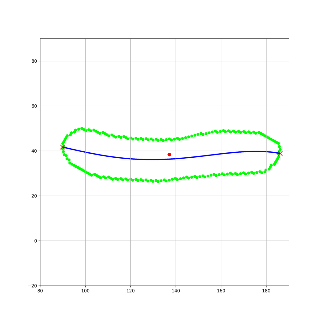
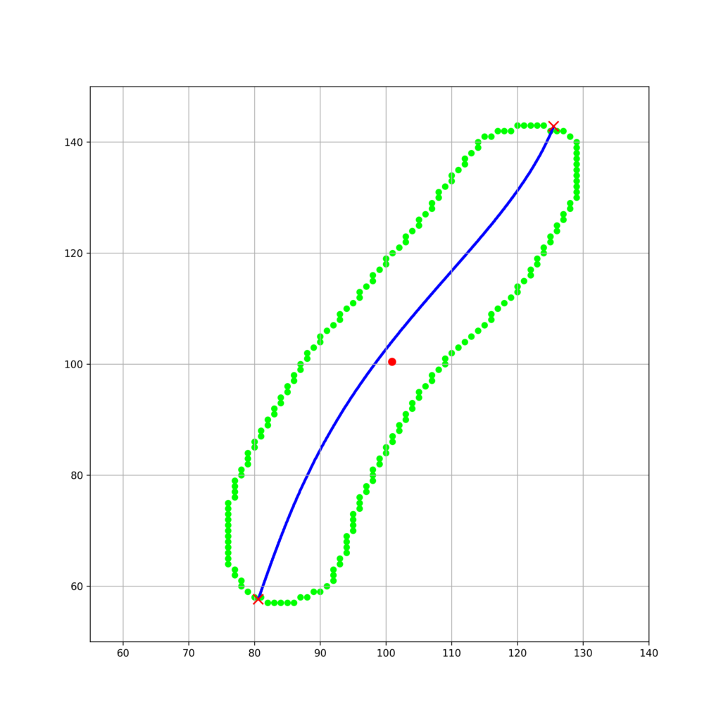
細胞軸を決定することができました。
これを基底逆変換してプロットしてみます。
fig_base_reverse_convert = plt.figure(figsize=(10,10))
line_reversed = [Q.transpose()@inv(Q.transpose()@Q)@np.array([j,i]) for i,j in zip(u_1,u_2)]
intersection_min = (min_u1,theta[0]*min_u1**4+theta[1]*min_u1**3 + theta[2]*min_u1**2+theta[3]*min_u1 + theta[4])
intersection_max = (max_u1,theta[0]*max_u1**4+theta[1]*max_u1**3 + theta[2]*max_u1**2+theta[3]*max_u1 + theta[4])
intersection_reverse_min = Q.transpose()@inv(Q.transpose()@Q)@np.array(intersection_min[::-1])
intersection_reverse_max = Q.transpose()@inv(Q.transpose()@Q)@np.array(intersection_max[::-1])
plt.scatter(intersection_reverse_min[0],intersection_reverse_min[1],s = 100,color = "red",zorder = 100,marker = "x")
plt.scatter(intersection_reverse_max[0],intersection_reverse_max[1],s = 100,color = "red",zorder = 100,marker = "x")
plt.xlim(55,140)
plt.ylim(50,150)
plt.grid()
plt.scatter([i[0] for i in cell],[i[1] for i in cell],s = 30,color = "lime")
plt.scatter(center[1],center[0],s = 50,color = "red",zorder = 100)
plt.scatter([i[0] for i in line_reversed],[i[1] for i in line_reversed],s = 3,color = "blue")
fig_base_reverse_convert.savefig("contours_base_reverse_convert.png",dpi=300)
実行結果