

以前、モンテカルロ法を使用して円周率を求めていた際、ピクセルを微小化していけば円周率の精度を上げながら求めていくことができるのではないかということに気づいたので、今回はそれを実装していってみたいとおもます。
上記の記事のように、面積比を使用することで円周率に迫っていきます。
目次
ピクセルの生成
まずは、それぞれの辺のピクセル数が2^nとなるような正方形を作成します。
import numpy as np
import random
import matplotlib.pyplot as plt
from tqdm import tqdm

array = np.zeros((int(2**i),int(2**i)))
r = int(int(array.shape[0])/int(2))
p,q = r,r
同時に半径、中心座標も求めることができます。
円の内外判定
円の内外判定には円の方程式を使用します。
以下の関数で、対象座標が円に含まれていればTrueを返します。
def is_within(x,y,radius,p,q):
    if ((x-p)**2 + (y-q)**2)< radius**2:
        return True
円周率の計算
面積比から円周率を計算します。
$$Pi_{est} = \frac{4True判定の座標数}{全座標数}$$
est_pi = 4*counter/(array.shape[0]**2)nに対する推定円周率のトラッキング
ここまでで、面積比から円周率を計算するアルゴリズムができましたが、nを1から増加させて行った時の推定円周率の変化をグラフにプロットして可視化してみます。
以下のようにコードを書き換えます。
import numpy as np
import random
import matplotlib.pyplot as plt
from tqdm import tqdm

def is_within(x,y,radius,p,q):
    if ((x-p)**2 + (y-q)**2)< radius**2:
        return True

fig = plt.figure()
plt.xlabel('m')
plt.ylabel('Estimated pi value')

for i in range(1,17):
    array = np.zeros((int(2**i),int(2**i)))
    r = int(int(array.shape[0])/int(2))
    p,q = r,r
    counter = int(0)
    for j in tqdm(range(array.shape[0])):
        for k in range(array.shape[0]):
            if is_within(j,k,r,p,q):
                counter += int(1)
            else:
                pass
    est_pi = 4*counter/(array.shape[0]**2)
    plt.scatter(i,est_pi,s = 4)
fig.savefig('pi_d.png',dpi=700)
実行結果
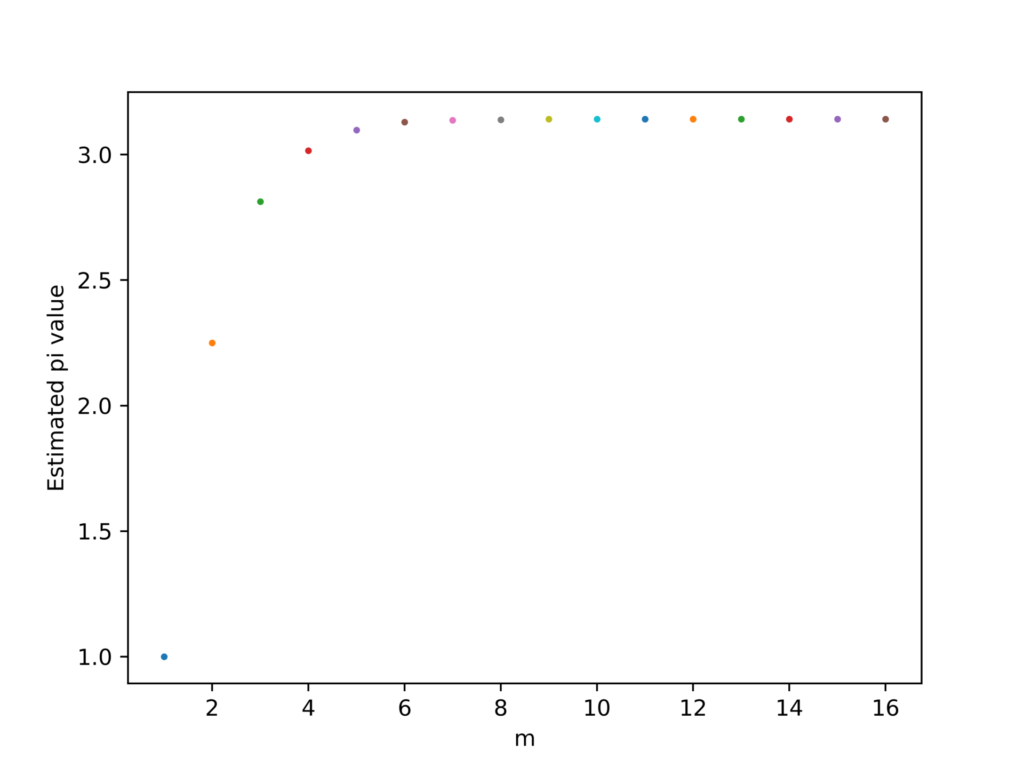
nが増加するほどある一定の値に漸近していっていることがわかります。このことから、計算量を増やせば増やすほど、正確な円周率を求められることがわかります。
アルゴリズムの高速化
上記のアルゴリズムでは、生成した二次元空間全域をループ毎に探索していました。そのため、nが1増加するごとに、探索時間は4倍に跳ね上がります。例えば、n=10の時、探索時間は3秒であったことを考えると、n=16の場合には50分を超えることになります。
この問題を解決するために、生成した二次元空間を4分割します。この時、面積比と円周率の関係は以下のようになります。
$$ \frac{True判定の座標数}{全座標数}= \frac{r^2Pi_{est}}{4r^2}$$
(rは結局打ち消されるので、探索範囲が1/4になるということはこの式からはわかりません。)
ここで、二次元空間の4分割をアルゴリズムに適用すると以下のようになります。
from itertools import count
import numpy as np
import random
import matplotlib.pyplot as plt
from tqdm import tqdm
import cv2

def is_within(x,y,radius,p,q):
    if ((x-p)**2 + (y-q)**2)< radius**2:
        return True

fig = plt.figure()
plt.xlabel('m')
plt.ylabel('Estimated pi value')

for i in range(1,17):
    array = np.zeros((int(2**i),int(2**i)))
    r = int(int(array.shape[0])/int(2))
    p,q = r,r
    counter = int(0)
    for j in tqdm(range(r)):
        for k in range(r):
            if is_within(j,k,r,p,q):
                counter += int(1)
            else:
                pass
    est_pi = 4*counter/(array.shape[0]**2)
    plt.scatter(i,4*est_pi,s = 4)

fig.savefig('pi_d.png',dpi=700)
計算結果の記録
nが増えるにつれて計算量が膨大となってしまうため、計算結果を後から再利用できるようにどこかに書き留めておく必要があります。
今回はopenpyxlモジュールを使用して、エクセルに計算結果を出力していきます。
エクセルの読み書きについては以下の記事にテンプレートを用意しています。
import numpy as np
import matplotlib.pyplot as plt
from tqdm import tqdm

import openpyxl
book = openpyxl.load_workbook('Book2.xlsx')
sheet = book['Sheet1']

def is_within(x,y,radius,p,q):
    if ((x-p)**2 + (y-q)**2)< radius**2:
        return True

fig = plt.figure()
plt.xlabel('m')
plt.ylabel('Estimated pi value')

for i in range(1,14):
    array = np.zeros((int(2**i),int(2**i)))
    r = int(int(array.shape[0])/int(2))
    p,q = r,r
    counter = int(0)
    for j in tqdm(range(r)):
        for k in range(r):
            if is_within(j,k,r,p,q):
                counter += int(1)
            else:
                pass
    est_pi = 4*counter/(array.shape[0]**2)
    sheet.cell(row=i,column=1).value = 2**i
    sheet.cell(row=i,column=2).value = est_pi*4
    #plt.scatter(i,est_pi,s = 4)

book.save('Book2.xlsx')
これで、アルゴリズムを一回実行すればその計算結果が保存されるため、結果を何度でも再利用することができます。
データの抽出
pythonで曲線近似を行うため、先ほどエクセルに出力したデータをpython上に戻す作業が必要です。
import openpyxl
import matplotlib.pyplot as plt
import numpy as np

book = openpyxl.load_workbook('Book2.xlsx')
active_sheet = book.active
column_1 = [active_sheet.cell(column=1, row=i+1).value for i in range(active_sheet.max_row)]
column_2 = [active_sheet.cell(column=2, row=i+1).value for i in range(active_sheet.max_row)]

print(column_1)
print(column_2)
column_n = [i for i in range(len(column_2))]

fig = plt.figure()
plt.scatter(column_n,column_2,s=3)
plt.plot(column_n,column_2)

fig.savefig('pi.png',dpi=700)
これらの操作で、nの値とその時の予想円周率を取得することができました。
次回の記事で、予想円周率とnの関係を非線形近似して色々試してみます。

