

方程式の数値計算の際に、ニュートン法を使うことがたまにあるので、一旦まとめておきたいと思います。
目次
アルゴリズム
ニュートン法のアルゴリズムは至ってシンプルで、以下の漸化式を実装するだけです。
$$x_{i+1}=x_i-\frac{f(x_i)}{\frac{df(x_i)}{dx}}$$
実装例
以下の関数について考えてみます。
$$f(t)=sin(\frac{1}{e^{t^2}}-t^{1.4})$$
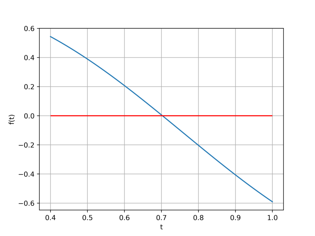
振動しているので解は無数にありますが、今回は定義域中の解について考えてみます。
初期値は左から近づける場合には0.4より大きく0.7より小さい数、右から近づける場合は1.0より小さく、0.71より大きい数を設定します。
import numpy as np
import matplotlib.pyplot as plt
#定義域、初期値を設定。
t_min,t_max =0.4,1
t_i = 0.5
#rはループを回す回数。
r = 10
#ここに任意関数を定義。
def f(t):
return np.sin(np.exp(-t**(2))-t**1.4)
#微分を行う関数
def N_R(t_i):
h = 10**(-9)
df_dt = (f(t_i+h)-f(t_i))/h
P_i = (t_i,f(t_i))
return -((P_i[1]-df_dt*P_i[0])/df_dt)
#グラフおよび収束の様子をプロット
t =np.linspace(t_min,t_max,1000)
f_t = f(t)
fig = plt.figure()
plt.plot(t,f_t)
for i in range(r):
t_i = N_R(t_i)
print(t_i)
if t_i < t_max and t_i > t_min:
plt.scatter(t_i,f(t_i),s=30)
plt.xlabel('t')
plt.ylabel('f(t)')
plt.hlines(0,t_min,t_max,color='red')
plt.grid()
fig.savefig('result.png',dpi=500)
>>>
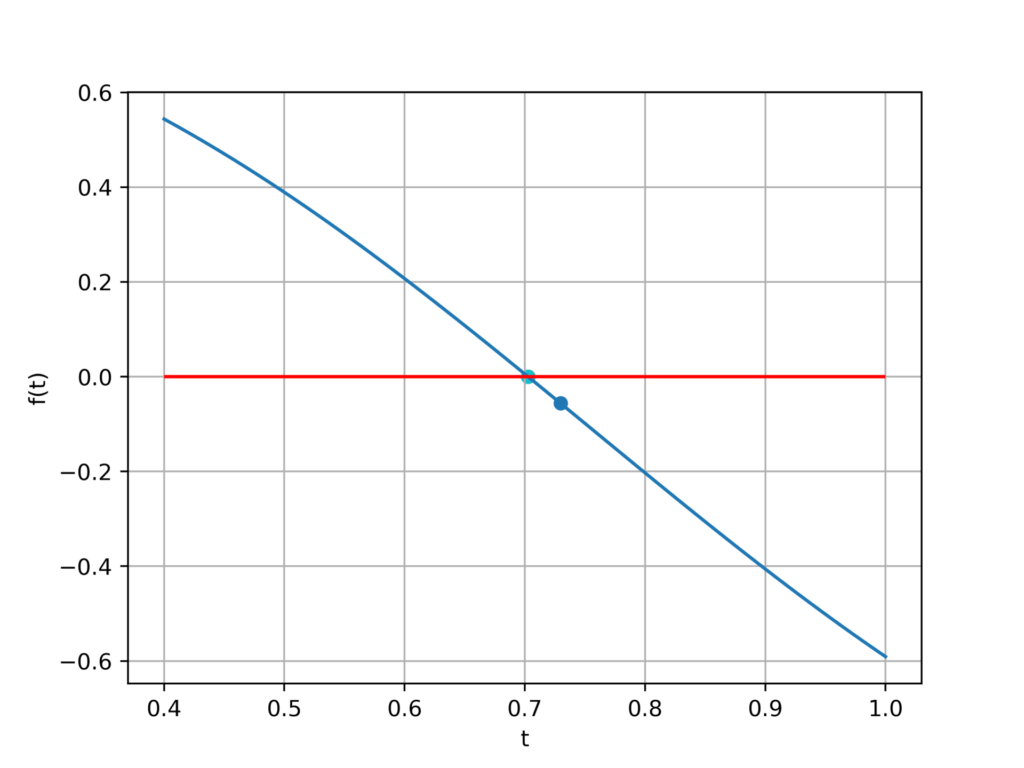
0.7297213736569597
0.7028316964147346
0.7027494520614176
0.7027494509107118
0.7027494509107121
0.702749450910712
0.702749450910712
0.702749450910712
0.702749450910712
0.702749450910712収束の速度が早いことがわかります。
平方根の計算
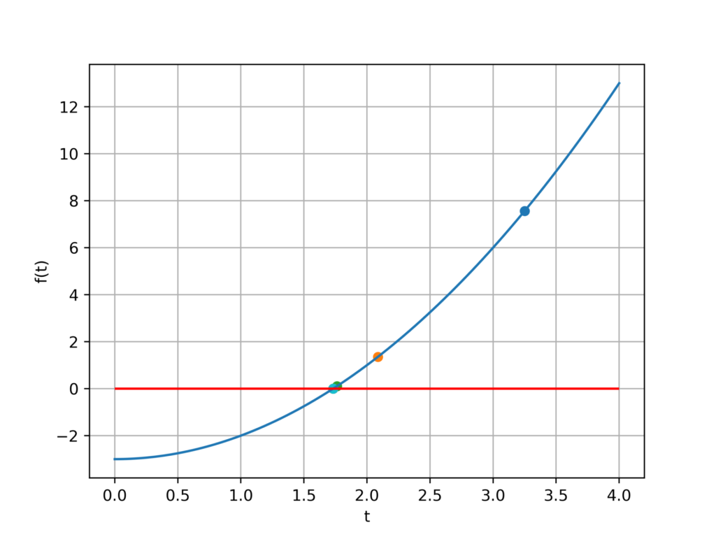
ニュートン法を利用すると平方根を計算することもできます。
関数を以下のように定義すれば、nの平方根を容易に求めることができます。
$$f(t)=t^2-n(\forall n>0)$$
import numpy as np
import matplotlib.pyplot as plt

t_min,t_max =0,4
t_i = 0.5
r = 10
n = 3
def f(t):
    return t**2-n

def N_R(t_i):
    h = 10**(-9)
    df_dt = (f(t_i+h)-f(t_i))/h
    P_i = (t_i,f(t_i))
    return -((P_i[1]-df_dt*P_i[0])/df_dt)

t =np.linspace(t_min,t_max,1000)
f_t = f(t)
fig = plt.figure()
plt.plot(t,f_t)
for i in range(r):
    t_i = N_R(t_i)
    print(t_i)
    if t_i < t_max and t_i > t_min:
        plt.scatter(t_i,f(t_i),s=30)
plt.xlabel('t')
plt.ylabel('f(t)')
plt.hlines(0,t_min,t_max,color='red')
plt.grid()
fig.savefig('result.png',dpi=500)
>>>
3.2499997724639984
2.0865385578036664
1.762163245582123
1.7323080942939666
1.7320508267053865
1.7320508075688787
1.7320508075688774
1.7320508075688774
1.7320508075688774
1.7320508075688774
出力結果
円周率の計算
円周率もニュートン法を用いて近似することができます。
例えば以下のような関数を定義するとします。
$$f(t)=sin(t)-\frac{1}{2}$$
この時、解の一つについて
$$t=\frac{\pi}{6}$$
となることを利用します。
import numpy as np
import matplotlib.pyplot as plt

t_min,t_max =0,2
t_i = 0
r = 10
n = 3
def f(t):
    return np.sin(t)-1/2

def N_R(t_i):
    h = 10**(-9)
    df_dt = (f(t_i+h)-f(t_i))/h
    P_i = (t_i,f(t_i))
    return -((P_i[1]-df_dt*P_i[0])/df_dt)

t =np.linspace(t_min,t_max,1000)
f_t = f(t)
fig = plt.figure()
plt.plot(t,f_t)
for i in range(r):
    t_i = N_R(t_i)
    print(t_i*6)
    if t_i < t_max and t_i > t_min:
        plt.scatter(t_i,f(t_i),s=30)
plt.xlabel('t')
plt.ylabel('f(t)')
plt.hlines(0,t_min,t_max,color='red')
plt.grid()
fig.savefig('result.png',dpi=500)
>>>
2.999999918312343
3.140666842865217
3.141592612385148
3.141592653589793
3.141592653589793
3.141592653589793
3.141592653589793
3.141592653589793
3.141592653589793
3.141592653589793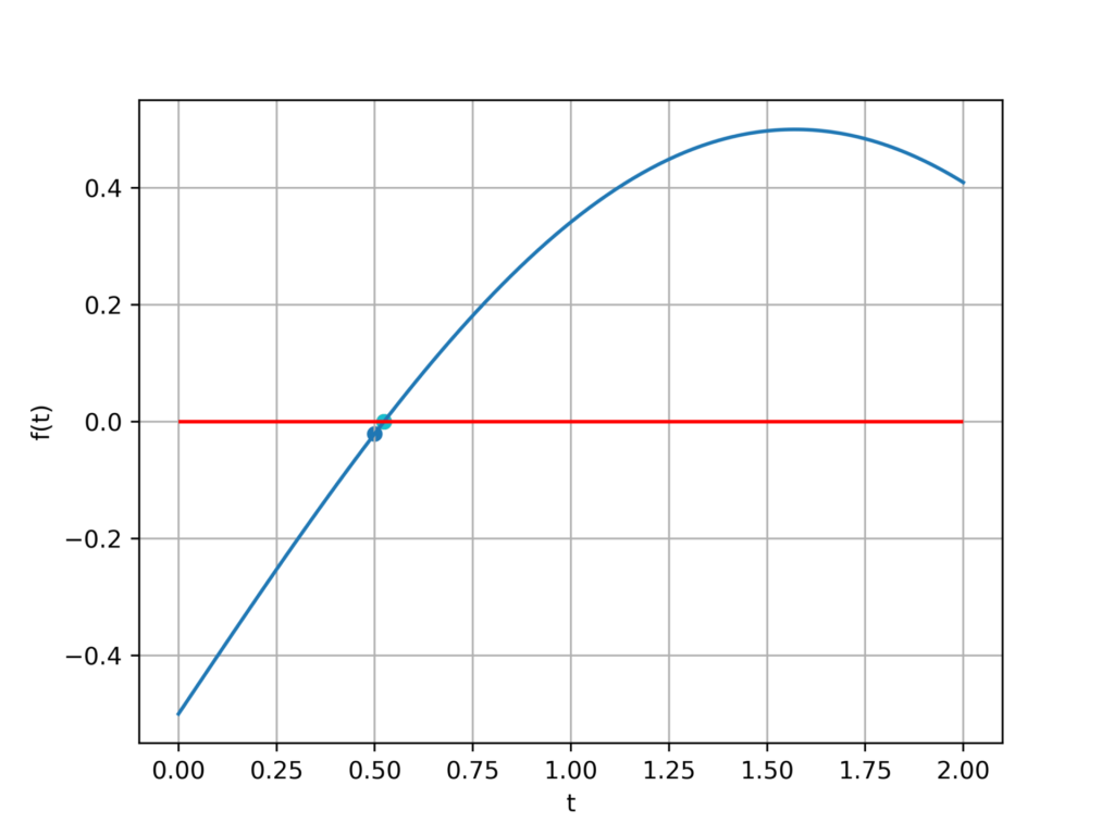
確率収束で対抗
ニュートン法の収束速度はかなり速い気がしますが、確率収束で対抗してみたいと思います。
アルゴリズム
まずはグラフから解が存在する範囲を定義します。
この範囲内の乱数を発生させ、解の左側で最も解に近いものと解の右側で最も解に近いものを次の乱数発生範囲とします。
これを繰り返していくことで、限りなく解に近い値を求めることができます。
import numpy as np
import random
import matplotlib.pyplot as plt

t_min, t_max = 0.25,0.75

def f(t):
    return np.sin(t)-1/2

t =np.linspace(t_min,t_max,1000)
f_t = f(t)

fig = plt.figure()
plt.hlines(0,t_min,t_max,color='red')
plt.plot(t,f_t)
plt.xlabel('t')
plt.ylabel('f(t)')
plt.grid()


for i in range(100):
    t_r = random.uniform(t_min,t_max)
    f_t_r = f(t_r)
    plt.scatter(t_r,f_t_r)
    if f_t_r<0 and t_r>t_min:
        t_min = t_r
    elif f_t_r>0 and t_r<t_max:
        t_max = t_r
    print(t_r*6)
fig.savefig('result_2.png',dpi=500)
>>>
---------90
3.1415926535897936
3.141592653589794
3.1415926535897936
3.1415926535897936
3.1415926535897936
3.141592653589794
3.141592653589793
3.141592653589793
3.1415926535897936
3.1415926535897936
ニュートン法よりは収束速度が遅いですが、確実に収束していっていることがわかります。
