

一般に、二変数での線形回帰を行う際には、L2ノルムを最小化するような直線を求めます。
この時に、正規方程式を使用して簡単に計算できることを学んだので、まとめておきます。
目次
正規方程式の作成
今回は以下のような変数を使用します。
X = [3, 6, 9, 12, 15, 18, 21, 24, 27, 30]
Y = [5, 8, 11, 20, 25, 31, 33, 43, 45, 51]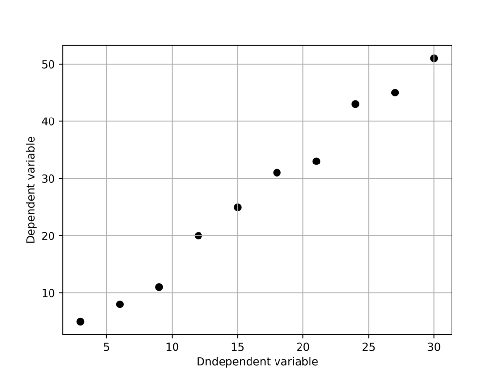
上記の二変数を使用して
$$\hat{f}(x) = ax+b$$
となる$A$と$B$を求めます。
この時の式は以下のように書くことができます。
$\begin {pmatrix}3&1\\\vdots&\vdots\\30&1\end{pmatrix} \begin {pmatrix}a\\b\end{pmatrix} =\begin {pmatrix}5\\\vdots\\51\end{pmatrix} $
簡略化すると、
$Ax = c$
となりますが、未知数に対する方程式の個数が多すぎるため、解を求めることができません。
そのため、以下のように正規方程式を作成して$e := |Ax-c|$を最小化するxを求めます。
$A^{\mathrm{T}}Ax =A^{\mathrm{T}}c$
Pythonで実装
import matplotlib.pyplot as plt
import numpy as np
from numpy.linalg import solve
fig = plt.figure()
X = [3*i for i in range(1,11)]
Y = [5,8,11,20,25,31,33,43,45,51]
print(X)
print(Y)
A = np.array([[i,1] for i in X])
c = np.transpose(np.array(Y))
A_t = np.transpose(A)
left = A_t@A
right = A_t@c
d = solve(left,right)
y_hat = [i*d[0]+d[1] for i in X]
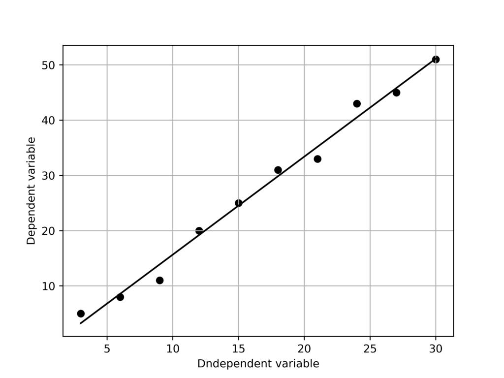
plt.scatter(X,Y,color = "black")
plt.plot(X,y_hat,color = 'black')
plt.xlabel("Dndependent variable")
plt.ylabel("Dependent variable")
plt.grid()
fig.savefig("a.png",dpi = 500)
>>>
[3, 6, 9, 12, 15, 18, 21, 24, 27, 30]
[5, 8, 11, 20, 25, 31, 33, 43, 45, 51]
[[3465 165]
[ 165 10]]
[5805 272]
[ 1.77373737 -2.06666667]実行結果
Numpy.polyfitと比較
Numpyで行った線形回帰との差を見てみます。
solve(left,right)
np.polyfit(X,Y,1)
>>>
[ 1.77373737 -2.06666667]
[ 1.77373737 -2.06666667]
同じなので、内部では同様のアルゴリズムを使用しているのかもしれません。
ランダムプロットで計算
大量のプロットをランダムに生成して線形回帰を行なってみます。
X = [i for i in range(1,100)]
Y = [random.randint(i-100,i+100) for i in X]
[0.7595671  9.33477633]
None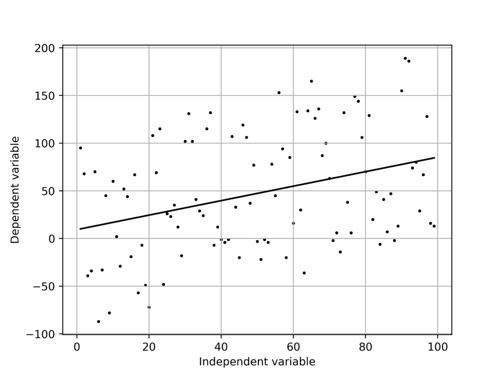
線形回帰のテンプレ
いつでも使えるように関数化しておきます。
import matplotlib.pyplot as plt
import numpy as np
from numpy.linalg import solve

def linear_regression(X:int,Y:int) -> None:
    A,c= np.array([[i,1] for i in X]),np.transpose(np.array(Y))
    A_t = np.transpose(A)
    left, right= A_t@A, A_t@c
    d = solve(left,right)
    y_hat = [i*d[0]+d[1] for i in X]
    plt.scatter(X,Y,color = "black")
    plt.plot(X,y_hat,color = 'black')
    plt.xlabel("Dndependent variable")
    plt.ylabel("Dependent variable")
    plt.grid()
    fig.savefig("linear_regression.png",dpi = 500)
