

pythonでグラフを扱える強力なモジュールであるNetworkXの基本的な操作方法をまとめておきます。
目次
インストール
ターミナルで以下のどちらかを実行します。
#homebrew
pip install network

#conda
conda install network
有向グラフオブジェクトの生成
import networkx as n
import matplotlib.pyplot as plt

#GraphD class
class GraphD:
    def __init__(self) -> None:
        #networkx object
        self.G = n.DiGraph()

#GraphD object
graphD = GraphD()
ここで生成したgraphDオブジェクトに対して操作を行なっていきます。
ノード、エッジの追加
#add a node
graphD.G.add_node(1)
#add nodes
graphD.G.add_nodes_from([i+1 for i in range(5)])

#add an edge 1->2
graphD.G.add_edge(1,2)

#add edges i->j
graphD.G.add_edges_from([(i,j) for i in range(1,5) for j in range(5,0,-1) if i != j])

#add a path 5->4->3->2->1
n.add_path(graphD.G, [i for i in range(5,0,-1)])
グラフ可視化
matplotlibを使用してグラフを可視化します。
n.draw(G, with_labels = True)
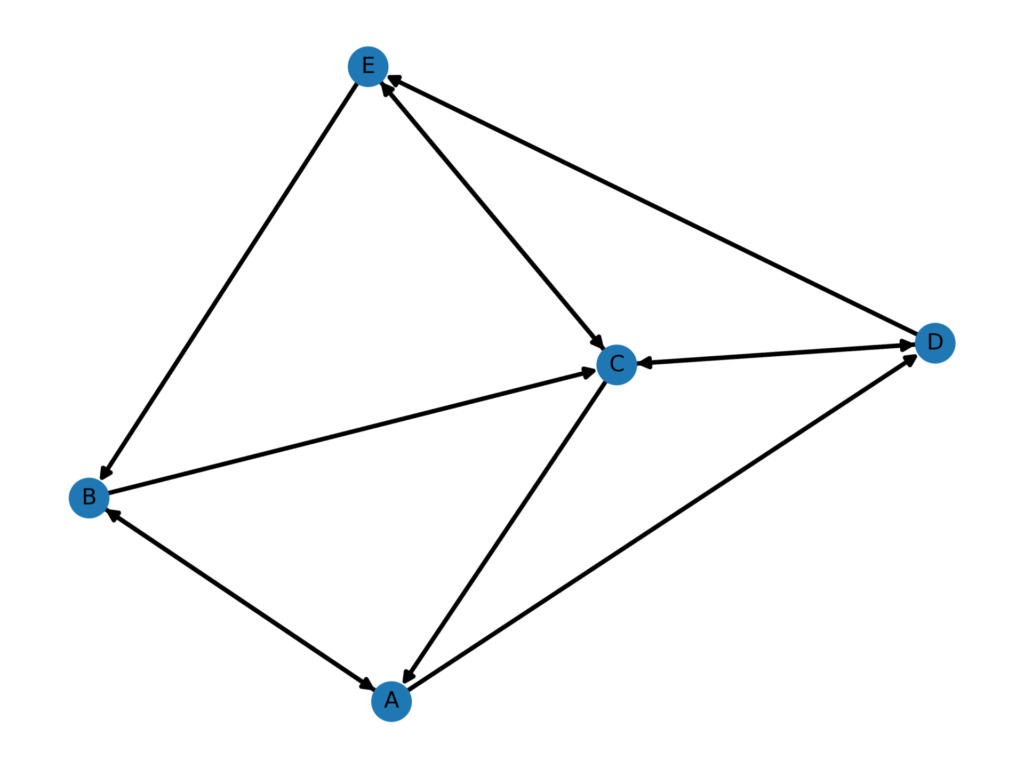
plt.show()隣接行列の可視化
以下の隣接行列をグラフに変換して可視化してみます。
draw parameters -> (with_labels = True,node_size = 300, width = 2,font_size = 10)#Mat_ADJ
,A,B,C,D,E
A,0,1,0,1,0
B,1,0,1,0,0
C,1,0,0,1,1
D,0,0,1,0,1
E,0,1,1,0,0
import networkx as n
import matplotlib.pyplot as plt
class GraphD:
def __init__(self) -> None:
#networkx object
self.G = n.DiGraph()
graphD = GraphD()
with open("adj.csv") as f:
adj = [[j.replace("\n","") for j in i.split(",")[1:]] for i in f.readlines()]
graphD.G.add_nodes_from(adj[0])
graphD.G.add_edges_from([((node,adj[0][c])) for i,node in enumerate(adj[0]) for c,j in enumerate(adj[i+1]) if int(j) == 1])
fig = plt.figure()
n.draw(graphD.G, with_labels = True,node_size = 300, width = 2,font_size = 10)
fig.savefig("result.png",dpi = 500)実行結果
ネットワーク特性値の取得
上記の隣接行列に対する各情報を取得していきます。
#nodes
print(graphD.G.nodes())
>>>
['A', 'B', 'C', 'D', 'E']

#edges
print(graphD.G.edges())
>>>
[('A', 'B'), ('A', 'D'), ('B', 'A'), ('B', 'C'), ('C', 'A'), ('C', 'D'), ('C', 'E'), ('D', 'C'), ('D', 'E'), ('E', 'B'), ('E', 'C')]

#degree
print(graphD.G.degree())
>>>
[('A', 4), ('B', 4), ('C', 6), ('D', 4), ('E', 4)]
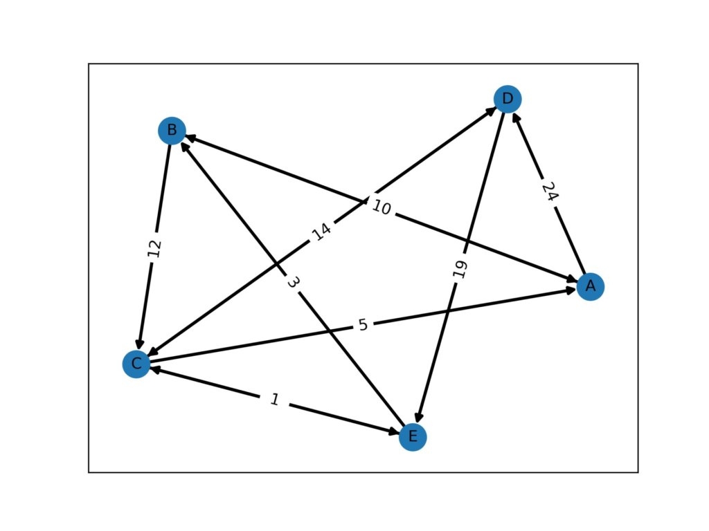
重み付き有向グラフ
隣接行列の値を任意の値にすることで重みを表現できます。
以下の隣接行列について重み付き有向グラフを可視化してみます。
adj.csv
,A,B,C,D,E
A,0,10,0,24,0
B,27,0,12,0,0
C,5,0,0,7,15
D,0,0,14,0,19
E,0,3,1,0,0


import networkx as n
import matplotlib.pyplot as plt

class GraphD:
    def __init__(self) -> None:
        #networkx object
        self.G = n.DiGraph()

graphD = GraphD()

with open("adj.csv") as f:
    adj = [[j.replace("\n","") for j in i.split(",")[1:]] for i in f.readlines()]

graphD.G.add_nodes_from(adj[0])
edges = {((node,adj[0][c])): int(j)  for i,node in enumerate(adj[0]) for c,j in enumerate(adj[i+1]) if int(j) != 0}
pos = n.spring_layout(graphD.G)
graphD.G.add_weighted_edges_from([(i[0],i[1],edges[i]) for i in list(edges.keys())])


fig = plt.figure()
n.draw_networkx_nodes(graphD.G, pos, node_size=300)
n.draw_networkx_edges(graphD.G, pos, width=2)
n.draw_networkx_labels(graphD.G, pos, font_size=10, font_color="black")
n.draw_networkx_edge_labels(graphD.G, pos, edge_labels={(i, j): w['weight'] for i, j, w in graphD.G.edges(data=True)})


fig.savefig("result.png",dpi = 500)
出力結果
周辺ノードの取得
接続されているすべての周辺ノードを取得します。
neighbors = list(set([i for i in n.all_neighbors(graphD.G,"A")]))
>>>
['D', 'B', 'C']
Dijkstra法による最短経路と経路長の取得
ダイクストラ法のアルゴリズムを実装するととんでもない時間がかかるため、ビルトインメソッドを使用します。
上記の隣接行列に対して、AからCまでの最短経路を求めてみます。
p = n.dijkstra_path(graphD.G, "A", "C")
pathway = [print(node,end="->") if i != len(p)-1 else print(node) for i,node in enumerate(p)]
length = n.dijkstra_path_length(graphD.G, "A", "C")
>>>
['A', 'B', 'C']
A->B->C
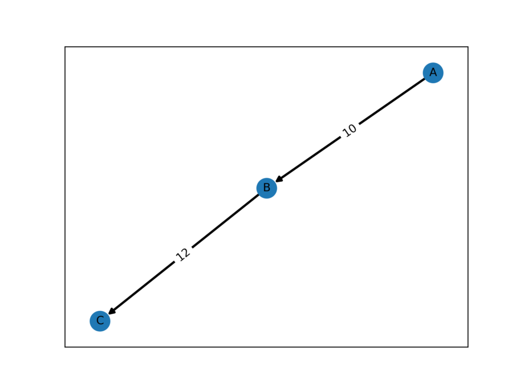
22グラフから最短経路のみを抽出
最短経路が求まったら、その結果を利用して取得した経路のみを抽出することもできます。
ここでは、最短経路と元のグラフから最短経路分を抜いたグラフの両方を可視化します。
最短経路の可視化
import networkx as n
import matplotlib.pyplot as plt

class GraphD:
    def __init__(self) -> None:
        #networkx object
        self.G = n.DiGraph()

graphD = GraphD()

with open("adj.csv") as f:
    adj = [[j.replace("\n","") for j in i.split(",")[1:]] for i in f.readlines()]

graphD.G.add_nodes_from(adj[0])
edges = {((node,adj[0][c])): int(j)  for i,node in enumerate(adj[0]) for c,j in enumerate(adj[i+1]) if int(j) != 0}
pos = n.spring_layout(graphD.G)
graphD.G.add_weighted_edges_from([(i[0],i[1],edges[i]) for i in list(edges.keys())])


fig = plt.figure()
graphP = GraphD()
nodes = n.dijkstra_path(graphD.G, "A", "C")
edges = [(nodes[i],nodes[i+1],edges[nodes[i],nodes[i+1]]) for i in range(len(nodes)-1)]

graphP.G.add_nodes_from(nodes)
graphP.G.add_weighted_edges_from(edges)

pos = n.spring_layout(graphP.G)


n.draw_networkx_nodes(graphP.G, pos, node_size=300)
n.draw_networkx_edges(graphP.G, pos, width=2)
n.draw_networkx_labels(graphP.G, pos, font_size=10, font_color="black")
n.draw_networkx_edge_labels(graphP.G, pos, edge_labels={(i, j): w['weight'] for i, j, w in graphP.G.edges(data=True)})

fig.savefig("result.png",dpi = 500)
実行結果
最短経路を除いたグラフ
import networkx as n
import matplotlib.pyplot as plt

class GraphD:
    def __init__(self) -> None:
        #networkx object
        self.G = n.DiGraph()

graphD = GraphD()

with open("book.csv") as f:
    adj = [[j.replace("\n","") for j in i.split(",")[1:]] for i in f.readlines()]

graphD.G.add_nodes_from(adj[0])
edges = {((node,adj[0][c])): int(j)  for i,node in enumerate(adj[0]) for c,j in enumerate(adj[i+1]) if int(j) != 0}
pos = n.spring_layout(graphD.G)
graphD.G.add_weighted_edges_from([(i[0],i[1],edges[i]) for i in list(edges.keys())])


for i in n.dijkstra_path(graphD.G, "A", "C"):
    graphD.G.remove_node(i)

fig = plt.figure()
n.draw_networkx_nodes(graphD.G, pos, node_size=300)
n.draw_networkx_edges(graphD.G, pos, width=2)
n.draw_networkx_labels(graphD.G, pos, font_size=10, font_color="black")
n.draw_networkx_edge_labels(graphD.G, pos, edge_labels={(i, j): w['weight'] for i, j, w in graphD.G.edges(data=True)})


fig.savefig("result.png",dpi = 500)
実行結果
元からノードが5つしかなかったので、こうなります。
三次元空間にプロット
使えるかどうかわかりませんが、三次元空間にプロットもできます。
import networkx as n
import matplotlib.pyplot as plt
import numpy as np
class GraphD:
    def __init__(self) -> None:
        #networkx object
        self.G = n.DiGraph()

graphD = GraphD()

with open("adj.csv") as f:
    adj = [[j.replace("\n","") for j in i.split(",")[1:]] for i in f.readlines()]

graphD.G.add_nodes_from(adj[0])
edges = {((node,adj[0][c])): int(j)  for i,node in enumerate(adj[0]) for c,j in enumerate(adj[i+1]) if int(j) != 0}
pos = n.spring_layout(graphD.G)
graphD.G.add_weighted_edges_from([(i[0],i[1],edges[i]) for i in list(edges.keys())])

fig = plt.figure()

n.draw_networkx_nodes(graphD.G, pos, node_size=100)
n.draw_networkx_edges(graphD.G, pos, width=1)
n.draw_networkx_labels(graphD.G, pos, font_size=7, font_color="black")
n.draw_networkx_edge_labels(graphD.G, pos, edge_labels={(i, j): w['weight'] for i, j, w in graphD.G.edges(data=True)})

fig.savefig("result.png",dpi = 500)


graph = graphD.G.to_undirected()


pos = n.spring_layout(graphD.G, dim=3)
arr = np.array([pos[n] for n in graphD.G])


fig = plt.figure(facecolor="w")
ax = fig.add_subplot(111,projection="3d")


ax.scatter(
    arr[:, 0],
    arr[:, 1],
    arr[:, 2],
    s=200,
)

for n in graphD.G.nodes:
    ax.text(*pos[n], n)

for i in graphD.G.edges:
    n0 = pos[i[0]]
    n1= pos[i[1]]
    ax.plot([n0[0], n1[0]], [n0[1], n1[1]], [n0[2], n1[2]], c="black")

fig.savefig('result3.png',dpi = 500)

Graphvizによる可視化
NetworkXと似たような可視化モジュールがPythonで使えるようなので、ついでにまとめます。
有向グラフ
以下の隣接行列に対応する有向グラフを作成します。
,A,B,C,D,E,F,G,H,I,J
A,0,10,0,24,0,0,0,0,0,0
B,10,0,0,0,0,0,0,0,0,10
C,0,0,0,7,0,0,0,0,0,0
D,0,0,14,0,0,19,0,0,0,0
E,0,20,1,0,0,0,10,0,13,0
F,0,0,0,0,0,0,0,0,0,0
G,15,0,0,0,0,0,0,0,0,20
H,0,4,0,0,0,0,0,0,0,0
I,0,0,0,0,0,0,0,0,0,0
J,0,0,0,0,0,0,0,0,0,0

from graphviz import Digraph

G = Digraph(format="png")
G.attr("node", shape="circle")

with open("adj.csv") as f:
    adj = [[j.replace("\n","") for j in i.split(",")[1:]] for i in f.readlines()]

edges = {((node,adj[0][c])): int(j)  for i,node in enumerate(adj[0]) for c,j in enumerate(adj[i+1]) if int(j) != 0}
edge_labels = list(edges.values())
for i,j in edges:

    G.edge(str(i), str(j))

G.render("G")
実行結果

重み付き有向グラフ
どうやら、重みラベルは正規化しないと受け付けてくれないようなので、重みの最大値を使用して正規化したラベルを使用します。
,A,B,C,D,E,F,G,H,I,J
A,0,10,0,24,0,0,0,0,0,0
B,10,0,0,0,0,0,0,0,0,10
C,0,0,0,7,0,0,0,0,0,0
D,0,0,14,0,0,19,0,0,0,0
E,0,20,1,0,0,0,10,0,13,0
F,0,0,0,0,0,0,0,0,0,0
G,15,0,0,0,0,0,0,0,0,20
H,0,4,0,0,0,0,0,0,0,0
I,0,0,0,0,0,0,0,0,0,0
J,0,0,0,0,0,0,0,0,0,0

from graphviz import Digraph

G = Digraph(format="png")
G.attr("node", shape="circle")

with open("book.csv") as f:
    adj = [[j.replace("\n","") for j in i.split(",")[1:]] for i in f.readlines()]


edges = {((node,adj[0][c])): int(j)  for i,node in enumerate(adj[0]) for c,j in enumerate(adj[i+1]) if int(j) != 0}
edge_labels = list(edges.values())
for i,j in edges:
    G.edge(str(i), str(j),label=str(edges[(i,j)]/max(edge_labels))[:4])

G.render("G")
実行結果
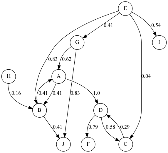
双方向接続の重みが違うところがありますが、これは適当に作ったからです。
